
Consolidating Excel Worksheets with Power Query
Adding together data scattered across many worksheets is a common Excel challenge. In this article we’ll show a clever and flexible way to tackle this using Power Query.
For those new to it, Power Query is Microsoft Excel’s tool for importing, cleaning and aggregating data. It is built into Excel and was created with the end business user in mind. With a little practice, it quickly becomes intuitive to setup and maintain.
Besides connecting to external data systems/files or the web, Power Query also gives us the ability to automatically consolidate and analyze data that resides within a workbook. There are many use cases for this including: rolling up weekly sales reports, consolidating employee time sheets, or even creating a consolidated project plan/schedule.
In our example we’ll cover consolidating department budgets into a single results table as, at the time of this writing, budget season is almost upon us.
Steps:
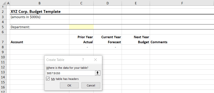
1. Create a data entry template
This will be the template that departments use to input their budgets. In the simple example below, we’re capturing the account, prior and current year amounts, and next year’s budget request, along with a column for comments.
- Convert the data entry section to an Excel table
Setup the column headings as you wish, and then hit Control-T to convert this to an Excel table. Tables are Excel’s functionality that make it easier to manage groups of related information.
- Format the table
Once converted to a table, you can also apply any formatting you like (borders, shaded header row, etc.) to make it more visually appealing for the end users.

- Name the table
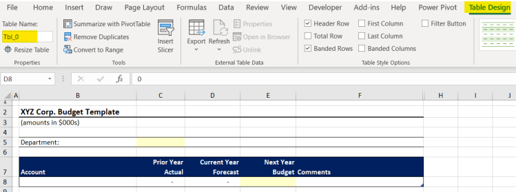
With any cell selected within the table, click on Table Design and note there is a box to key in a Table Name, as shown below. Name the table Tbl_0. As you’ll see later on, this naming is a key step to automating the data consolidation.
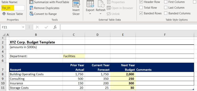
2. Copy and populate the data entry template
With the blank template now setup, make a copy of the worksheet and fill it in for a department (i.e., so that in this one file you will have multiple tabs – one per department). The example below shows a fictitious Facilities department budget. Note that when copying the worksheet, Excel automatically renamed the table for us. It keeps the “Tbl_” prefix from the template and increments it; again, you’ll see soon why this is important for automating the roll up (note that the actual number Excel gives it doesn’t matter; just the prefix needs to match).
Make another copy of the template and fill it in. Below is an example for the Finance department:

In reality, of course, you would likely have many more departments – for illustrative purposes, we’ll stop for now with only two. However, the real power of this consolidation technique is that it can be scaled for as many departments as necessary, with no additional maintenance or manual work.
3. Create a Power Query to consolidate the department budgets into one results table
This is where the magic happens!
- Create a blank query
Start by going into the Data tab on the menu bar and, in the Get & Transform Data section, select Get Data, From Other Sources and, finally, Blank Query:
- Connect the query to the contents of your Excel file
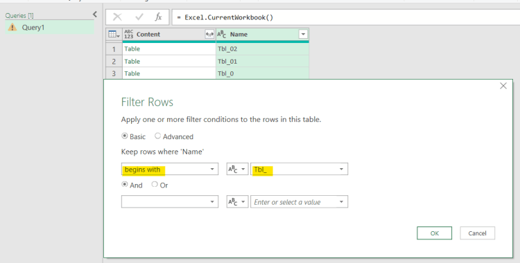
In the screen that appears next, type = Excel.CurrentWorkbook() in the formula bar and hit the Enter or the checkmark icon. This tells Power Query to connect to your Excel file itself, rather than an external data source:
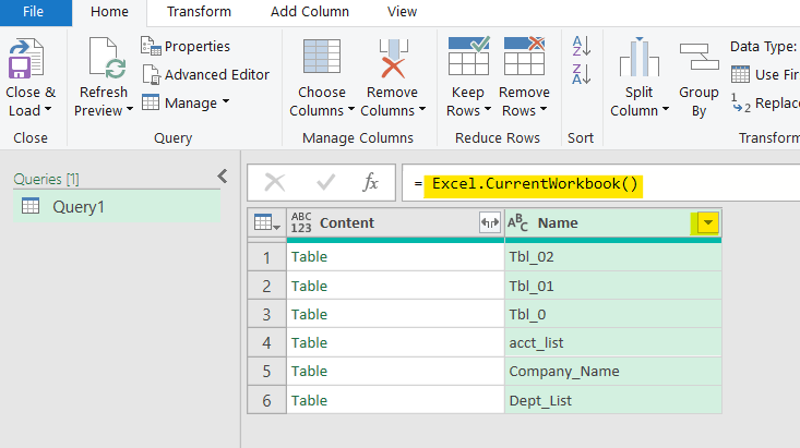
This brings up a window listing all the content with the workbook. From here we will filter the list so that we only connect to tables beginning with “Tbl_” (i.e., our data entry sheets). To do this, hit the filter arrow in the Name column heading, and then key in the filter details as below and hit OK:
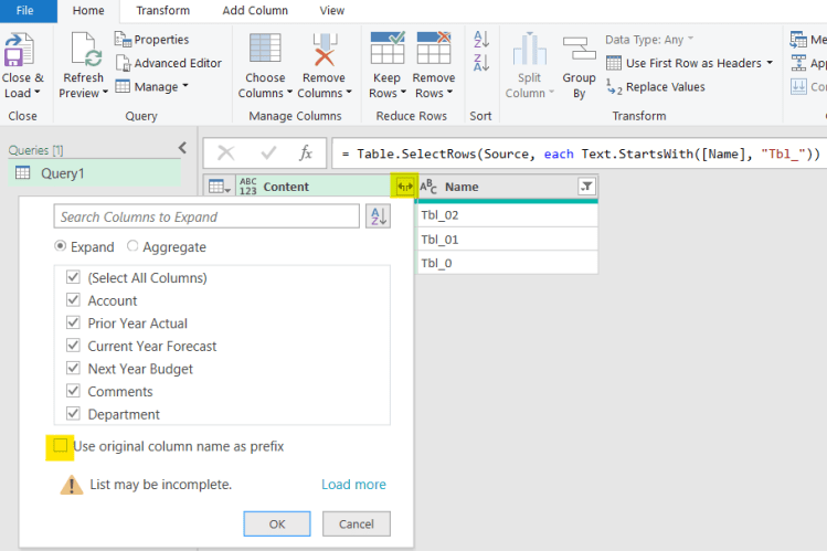
Next, we need to tell Power Query which columns we want to pull from these tables. This is done by hitting the “Expand” arrows in the Content column header. As shown below, you can pick and choose which columns you’d like to include (in this example we’ve selected all); just be sure to uncheck the “use original column name as prefix” box. Keeping it unchecked allows Power Query to append (i.e., combine) all the individual data entry tables.
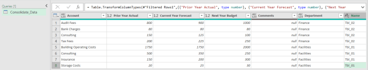
After hitting OK you’ll be presented with a preview of the combined table, including all rows from the Facilities and Finance budget tables. To clean it up a bit, we’ve filtered the Account field to exclude the table named Tbl_0 (the original blank template). There is no harm in keeping it included, but it will result in a blank row that’s unnecessary at the bottom of the table.
4. Output the Power Query results back into your workbook
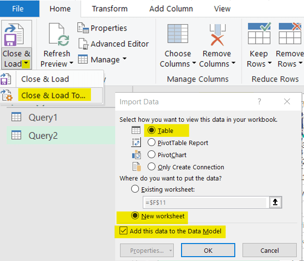
To this point we’ve been combining and previewing the data “under the hood” in Power Query. Now we need to make the combined data visible and useable in the body of the Excel file. To do this, hit the down arrow next to Close & Load, select Close & Load To…, and select Table and Add this Data to Data Model:
After you hit OK, Power Query will add a new worksheet to your file with a new consolidated table, pulling together all of the rows from the individual data entry tables:
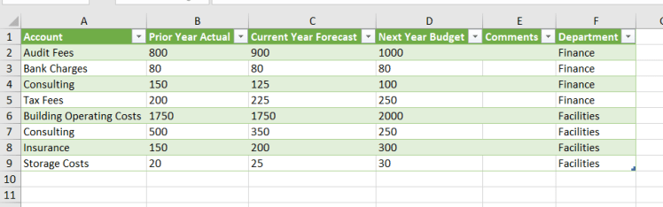
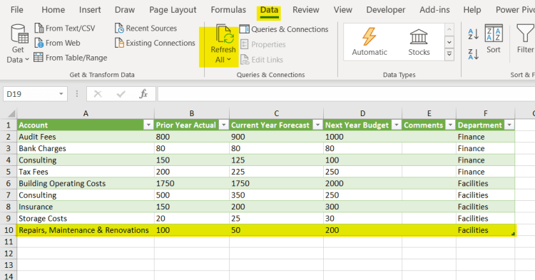
This table can be refreshed at any time by right-clicking in the table and selecting Refresh or, alternatively, by clicking Data and Refresh All in the Excel menu bar.
This makes the consolidation quite powerful and scalable as it will automatically bring in any new data that is entered.
For example, imagine the Facilities department missed budgeting for repairs and maintenance. If you input a budget for that account on their sheet and then refresh the consolidated table, it will flow in automatically:
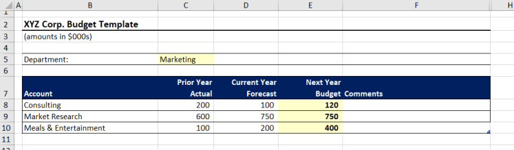
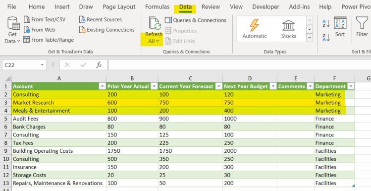
Similarly, if additional copies of the template are made and budgets established for more departments, those will also roll-up into the consolidated table (after hitting Data – Refresh All). Power Query knows to include these new tables because we’ve setup the file to name the tables beginning with “Tbl_” and this is the filter setup in the Power Query. In the example below we keyed in a budget for Marketing and then refreshed the table:
(Source budget)
(Resulting consolidated table after refresh)
Further Possibilities
Of course, because this produces an Excel table, you can perform calculations against it or even create pivot tables from it to perform further analysis or reporting.
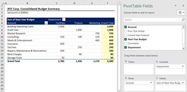
One common use case would be to create a pivot table report. One of our favourites at budget time is an expense matrix, showing accounts down the side and departments across the top, sorted from highest to lowest spend (example below). This is easily created from the consolidated table, and is dynamic, as it will refresh along with any changes made to the underlying data.
Closing Thoughts
Adding together data scattered across many sheets is a common Excel challenge. The technique detailed in this article can be used to roll up any data that you require. The three keys to automating it are:
- Having the source data in a consistent format (e.g., by creating a template)
- Formatting your template as an Excel table
- Following a consistent naming convention for tables (Excel looks after this for us as long as we’re careful about how we name the template table)
We hope this little trick helps simplify some of your repetitive Excel consolidations. Let us know how you apply it in your organization!
