Power Query Basics – Automating a Foreign Exchange Rate Feed in Excel

Power Query Basics – Automating a Foreign Exchange Rate Feed in Excel

Power Query is Microsoft Excel’s tool for easily importing, cleaning and aggregating data. It has been a game changer for how we approach financial modeling, particularly when working with large datasets. Power Query is easy to learn and maintain, as it shows each step of the process which you can review or adjust later. It’s also repeatable and highly automated as, once you set it up, everything done in Power Query can be refreshed on-demand with a couple of clicks.

In this article, we’ll walk through how to build an Excel spreadsheet using Power Query to pull foreign exchange rates from the Bank of Canada’s website (the same techniques can be used for importing data from other sources such as the US Federal Reserve). Even if you’ve never used Power Query before, in 15 minutes or less you’ll get a basic understanding of the tool and be left with a useful automated exchange rates spreadsheet.

Steps:

1. Create the connection to the Bank of Canada’s website

Power Query can connect to a variety of sources including Excel files, CSV/text files, PDFs and websites. The first step when creating a Power Query is to tell the spreadsheet where the source data resides (i.e., create a “connection” to it).

The Bank of Canada publishes a CSV file each day on its website containing daily exchange rates going back to 2017 for about two dozen currency pairs. This is the source that we use in this example, and the URL is:

https://www.bankofcanada.ca/valet/observations/group/FX_RATES_DAILY/csv?start_date=2017-01-03

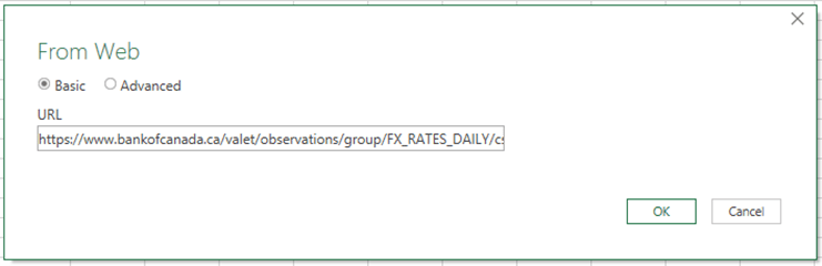
To create the connection, go into the Data tab on the menu bar and, in the Get & Transform Data section, click on the From Web section:

In the window that appears next, paste in the URL from above and click OK:

This will bring up a preview of the exchange rates file from the Bank of Canada’s website:

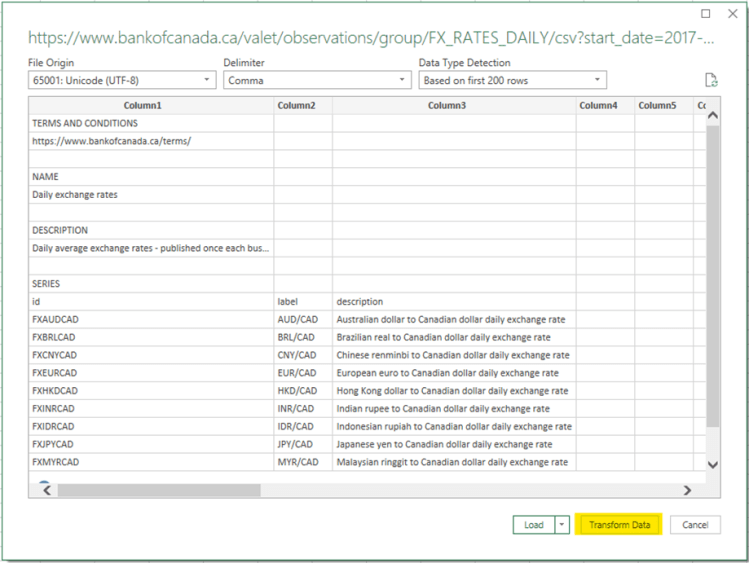
Click on Transform Data and we will do some simple adjustments to the data before loading it into Excel.

2. Transform the data

Here we will remove extraneous information and reformat the data so that it is easier to work with in our spreadsheet.

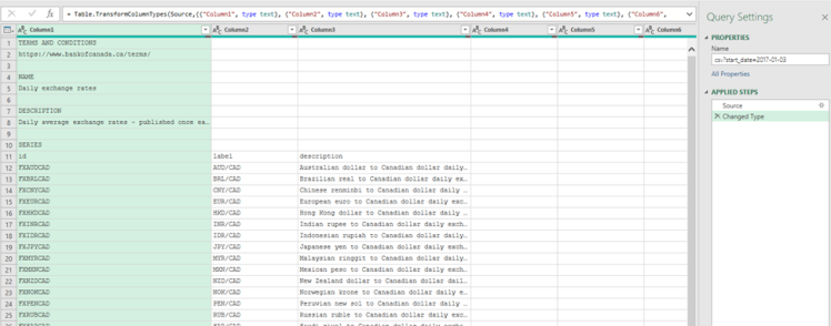
Once the query is loaded, you’ll see the following window – this is Power Query’s user interface:

• Rename query

Give the query a more intuitive name (e.g., “BOC Rates”) by typing over the entry in the Name section on the pane on the right side of the screen, and hitting Enter.

• Remove rows from the top of the CSV file

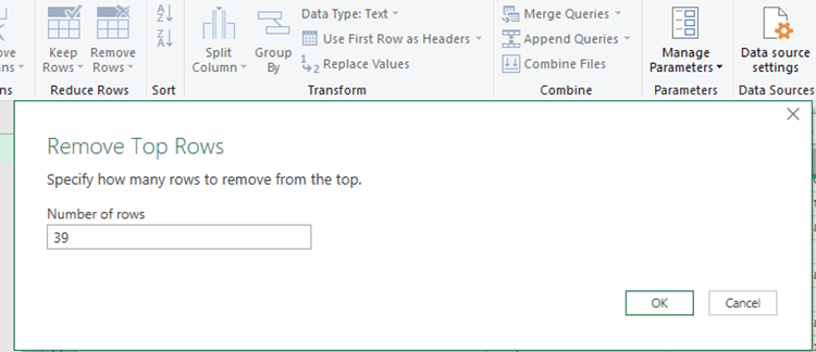
If you scroll down in the preview, you’ll see that the actual exchange rate data starts on row 40 of the file. The preceding rows just contain text explaining what each currency pair is, etc., and can be removed.

• To remove the unnecessary rows, click on Remove Rows from the menu bar, select Remove Top Rows and in the window that appears, specify that you would like to remove 39 rows from the top of the file and hit OK:

• Tell Power Query to use the first row as headers

Now the first row of the preview window should say  “date”, “FXAUDCAD”, “FXBRLCAD”, etc., with the dates and values appearing from row 2 onward. Click Use First Row as Headers in the Transform section of the menu bar.

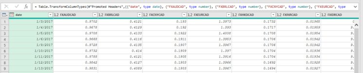
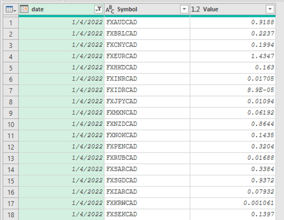
• Power Query will now promote what was the first row to the column headers, and the data will now begin on row 1. After this step, the preview window should look like this:

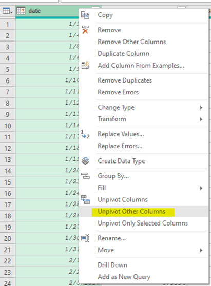
• “Unpivot” the values columns

Right now there are a lot of columns (i.e., fields) to deal with in this file. A more typical data structure that would be much easier to work with would be to have only three fields: date, value and currency pair – therefore resulting in each data point being an individual record.

“Unpivoting” is a powerful and often-used transformation feature built into Power Query. To use it, simply select the date column (by right-clicking on the date column header) and in the window that appears, select Unpivot Other Columns:

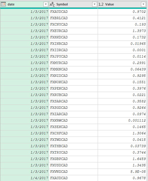
You’ll now be left with three fields: date, Attribute, and Value. For clarity, we’ll rename the Attribute field to Symbol, by double-clicking on the Attribute column header and typing over it.

3. Filter the data

You probably don’t want 5+ years of daily rates and every currency pair, so we’ll do some basic filtering before loading the data to Excel. To demonstrate this, we’ll assume that you only want rates after Dec. 31, 2021 and only for AUD, EUR and USD.

• Filter dates
  • Click the arrow next to the date header, then Date Filters and After:

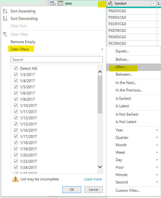
In the window that appears, select December 31, 2021 and hit OK. You will see the preview window update immediately, applying this filter:

• Filter currency pairs

Similarly, click the arrow next to the Symbol header. In the window that appears, uncheck (Select All), check off the currencies that you want to include in the spreadsheet (i.e., FXAUDCAD, FXEURCAD and FXUSDCAD) and hit OK:

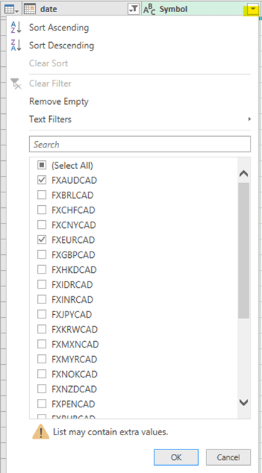
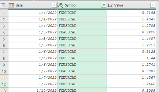
As with the date filter, the preview window will immediately apply the Symbol filter, so you are just left with the relevant currencies:

4. Load the data into Excel

Finally, hit the Close & Load button in the menu bar, this will close the Power Query editor, and bring you back to Excel, where it will automatically create a table containing the data from your query:

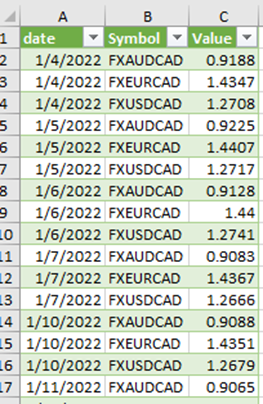
You now have a clean table of rates that can be refreshed at any time by right-clicking in the table and selecting Refresh or, alternatively, by clicking Data and Refresh All in the Excel menu bar. Each time you hit refresh (using either method), it will go back to the Bank of Canada’s website, pull the current CSV file and automatically apply all of the transformations that we defined in steps 2 and 3.

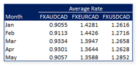
Of course, because this is an Excel table, you can perform calculations against it or even create pivot tables from it to perform further analysis. One common use case would be to create a simple pivot table calculating monthly average rates, similar to:

Closing Thoughts

This article scratches the surface of Power Query’s functionality. The power of the tool lies in its simplicity and ability to automate repetitive data importing, cleaning and aggregation tasks. We hope this introduction spurs your interest in exploring it further.

Let us know some of your organization’s data challenges and topics that you’d like to see covered in future articles.